Performance of Operational Fire Spread Models in California

Background:

Wildfires are a natural disturbance that shape the ecosystems and landscapes (Pausas and Keeley 2009) although they are a growing threat to the environment, economical assets and population in many regions worldwide (Molina-Terrén et al. 2019). In fact, substantial amounts of financial resources have been invested in fire management aiming to reduce the damage associated with unintended consequences of wildfires and improve safety for the population (Cardil and Molina 2015; Stocks and Martell 2016). Fire agencies rely on suites of wildfire analysis products that are designed to meet the needs of operational response and mitigation planning. Given the challenges that first responders and decision-makers were faced with to adequately predict fire spread and potential impacts, and dispatch the most appropriate resources every time a wildfire is detected in California, California Department of Forestry and Fire Protection (CAL FIRE) (2019), through a request for innovative ideas in March 2019, selected Wildfire Analyst Enterprise (WFA-e) to evaluate initial attack fires and calculate wildfire risk based on automatic simulations.

Wildfire simulators allow estimating fire spread and behaviour in complex environments, supporting planning and analysis of incidents in real time. However, uncertainty derived from input data quality and model inherent inaccuracies may undermine the utility of such predictions. Therefore, a validation of model’s performance in real incidents was needed.  

Aims: 

The main objective of this study was to assess the performance of fire spread models for initial attack incidents used in California through the analysis of the ROS of 1853 wildfires. 

Methods:  

We used the observed fire growth from the FireGuard (FG) database, ran an automatic simulation with Wildfire Analyst Enterprise and assessed the accuracy of the simulations by comparing observed and predicted ROS with well-known error and bias metrics, analysing the main factors influencing accuracy. Recent advances in technology have allowed monitoring the fire progression of most wildfires every 15 min in the United States of America (USA) through FG polygons (Figure 1). These data, when available for use on a fire, provide unprecedented capabilities to analyse factors influencing fire behaviour and compare the observed and predicted rate of spread (ROS) in fires distributed across different and complex landscapes. The product provides a set of independent polygons representing sections of the fire front. 

Figure 1: Wildfire ignitions retrieved from FireGuard in California from October 2019 to November 2021. Each fire has an associated rate of spread (ROS) for the first burning period (up to 8 h) obtained by averaging the ROS of all FG polygons by incident. The zoomed-scale box shows three fires with the associated FG polygons for the burning period (the largest fire is the Mountain View fire). 

To classify polygons into individual incidents (fires), we use a grid-growing clustering algorithm (Figure 2; Zhao et al.2015). All polygon centroids are projected into a 3D grid covering the spatio-temporal dimensions of the dataset using a 3 km in space and 24 h in time cell size resolution. This process leads to a density 3D matrix representing the number of elements at each cell. 

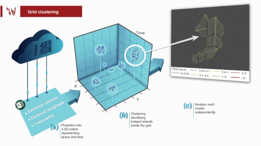
Figure 2. Extraction of ROS vectors from the FireGuard (FG) dataset: (a) retrieval and storing of the FG data in a database; (b) projection of FG polygons into a 3D matrix representing space and time. Clustering identification of hotspot islands inside the grid. (c) Example of a wildfire that shows the evolution in time of a set of FG polygons with their associated maximum ROS vector (bold line), the secondary spread vectors, and the overall perimeter (dashed yellow line). Vector colours are based on their ROS.

Once all clusters are identified, polygons in each incident are ordered in time, increased in resolution (number of vertices), and trimmed down to remove overlapping sections with previous polygons in time. Then a parent–child hierarchy of polygons is constructed based on the Hausdorf distance of each polygon with respect to the surrounding ones. More explicitly, we compute and identify the vertices leading to the maximum distance from a point in a polygon to the closest point in the surrounding ones. If the child polygon is in contact with other polygons, the Hausdorf distance is computed only with respect to those shared vertices. If the child polygon is not in contact with any other polygon, it is assumed that it was created by spotting, and the Hausdorf distance is computed with respect to all polygons within the last 8 h. Polygons that have no valid distance vector are considered to be independent ignition sources not caused by any other polygon. The maximum ROS vector of a polygon is given by the Hausdorf distance vector divided by the arrival time difference between the parent and child polygon. Once the parent–child hierarchy is established, we can also compute all secondary spread vectors by computing the minimum distance from each vertex of the source polygon to the target one divided by the elapsed time between them. 

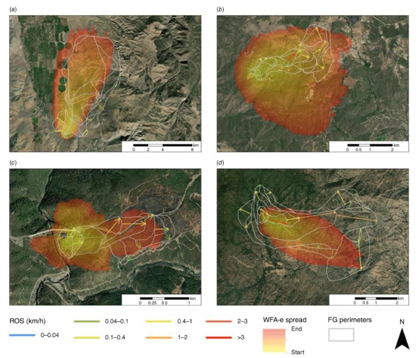
Figure 3: Fire progression (FireGuard data) and simulation of four wildfires through Wildfire Analyst Enterprise (WFA-e) in California: (a) Mountain View fire (lat.  38.515; lon.  −119.465; 2020/11/17); (b) Chaparral fire (lat.  33.485; lon.  −117.399; 2021/08/28); (c) Bridge fire (lat.  38.921; lon.  −121.037; 2021/09/05); (d) French fire (lat.  35.687; lon.  −118.55; 2021/08/18); note that the FG polygons and WFA-e simulated fire progression have the same time duration. 

We compared the ROS predicted by WFA-e and observed through FG based on four different well-known metrics (Cruz et al. 2018): (1) ROS residual representing the difference between the predicted and observed ROS. Therefore, a positive residual indicates an overestimation; (2) mean absolute error (MAE), representing the average of the absolute error; (3) mean bias error (MBE), representing the average bias between the predicted and observed values; (4) mean absolute percentage error (MAPE), a measure of prediction accuracy of a forecasting method in statistics that expresses the accuracy in relative terms. 

Key results:  

This work concludes that the fire spread model’s performance for California is in line with previous studies developed in other regions and the models are accurate enough to be used in real-time operations, especially with the use of adjustment modes that allow the calibration of predictions using field data. The accuracy of fire behaviour outputs is modulated by environmental conditions, especially fuel types and wind speed, which may bias ROS predictions. However, we also recognise that there are challenges regarding the effect of pyroconvection on local wind fields and the estimation of ROS in timber areas. The results of this evaluation suggest that the accuracy of fire simulations may be improved with newer models aiming to address the spread of fires in timber areas, crown fire behaviour modelling and the effect of pyroconvection in weather conditions and fire behaviour. Our approach addresses issues arising from the use of long fire runs, encompassing at times variations in fuel types, the estimation of fuel characteristics across the landscape, and the averaging of wind speed over broad spatial and temporal scales.  

Implications:  

This work allows users to better understand the performance of fire spread models in operational environments and opens new research lines to further improve the performance of current operational models. 

In TEMA project, the more accurate the simulation results are, the better response can be given through the platform to the operational firefighting team, increasing safety and reducing risks and human and material losses. 

Bibliography:

California Department of Forestry and Fire Protection (CAL FIRE) (2019) Request for Innovative         Ideas         (RFI2) Wildfire         Management.         Available          at: https://caleprocure.ca.gov/event/3540/0000012234 [last accessed 3 October 2023] 

Cardil A, Molina DM (2015) Factors Causing Victims of Wildland Fires in Spain (1980– 2010). Human and Ecological Risk Assessment: An International Journal 21, 67-80. 

Cruz MG, Alexander ME, Sullivan AL, Gould JS, Kilinc M (2018) Assessing improvements in models used to operationally predict wildland fire rate of spread. Environmental Modelling & Software 105, 54-63. 

Molina-Terrén DM, Xanthopoulos G, Diakakis M, Ribeiro L, Caballero D, Delogu GM, Viegas DX, Silva CA, Cardil A (2019) Analysis of forest fire fatalities in southern Europe: Spain, Portugal, Greece and Sardinia (Italy). International Journal of Wildland Fire 28, 85-98. 

Pausas JG, Keeley JE (2009) A burning story: the role of fire in the history of life. BioScience 59, 593-601. 

Stocks BJ, Martell DL (2016) Forest fire management expenditures in Canada 1970– 2013. The Forestry Chronicle 92, 298-306. 

Zhao Q, Shi Y, Liu Q, Fränti P (2015) A grid-growing clustering algorithm for geo-spatial data. Pattern Recognition Letters 53, 77-84.