Concept Activation Vectors from a Statistical Learning Perspective

Concept Activation Vectors (CAVs) [1] provide a quantitative framework for interpreting deep neural networks by measuring the sensitivity of model predictions to high-level, human-defined concepts. CAVs are powerful in safety-critical tasks - such as detecting wildfires and monitoring flood waters. By training simple linear probes on latent activations, CAVs reveal which visual features (smoke/flame patterns, river outlines) drive a model’s decisions, guiding both model debugging and dataset design.

Concept Activation Vectors

A CAV for a concept C at network layer l is obtained by training a linear classifier (e.g., ridge regression) to distinguish activations representing the presence vs. absence of C. The resulting weight vector  defines the concept direction. The sensitivity score  measures the directional derivative of the output logit for class k along  , indicating how much the concept influences the prediction on input x.

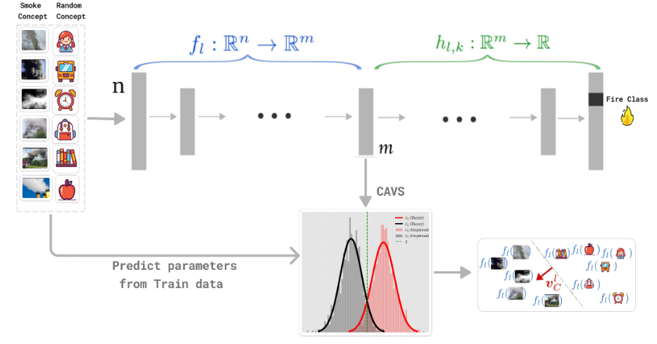
Putting it all together, the below Figure (derived from [1]) walks you through the CAV pipeline - from raw image patches all the way down to class-level sensitivity distributions - so you can see at a glance how the smoke concept plugs into a trained network and how its influence is quantified on predicting the class “fire”. We were able to estimate the Gaussian densities (μ and Σ) directly from the train data features’ vectors.

Ridge Regression CAV

To compute a Ridge CAV, we collect latent activations from:

• Concept-positive examples (e.g. patches with wildfire smoke)
• Concept-negative examples (e.g. smoke-free forest scenes)

Stacking features into X and labels into y, we solve:

Under high regularization (large λ) and equal sample sizes, this aligns closely with the simpler Pattern CAV introduced in  [2]​, where  and  are the mean activations for concept-positive and concept-negative samples, respectively.

Probabilistic Analysis of CAVs

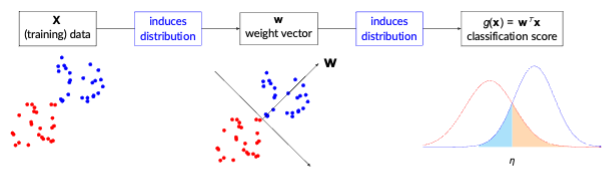
Modelling the classification score as Gaussian-distributed for each class, we can analytically predict classification accuracy and error rates [3]. Assuming  for non-concept and  for concept, the overall error combines misclassification probabilities weighted by class priors. This explains how concept separability depends on both mean shifts (e.g. smoke vs clear sky) and covariance structure (texture variability in flooded areas).

Practical Insights

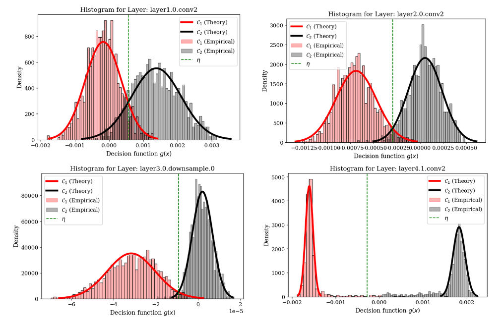
For each layer l (from layer1.0.conv2 to layer4.1.conv2) of a ResNet-18 model we plot the empirical histograms of the activations for concept-positive (red) versus random (gray) images, alongside the Gaussian densities predicted by our analytical solution (which is based on the Random Matrix Theory [4]) and the optimal threshold η (green dashed line).

The overlaid theoretical curves achieve an excellent fit to the empirical histograms at every depth, validating the model’s accuracy. Moreover, the progressive increase in peak separation - from shallow to deep layers - demonstrates that class separability steadily improves with network depth, reflecting the growing abstraction of high-level “smoke” features.

Dependency on Non-Concept Distribution

The very choice of “non-concept” samples used to fit the CAVs can dramatically change both the mean and spread of the TCAV scores - even though the concept class itself remains fixed. The Figure below illustrates this on Layer 1 activations for three signal classes on a toy task:

- Class 1 (low-freq, low-amp “non-concept”)
- Class 2 (low-freq, high-amp “non-concept”)
- Class 3 (high-freq “concept”)

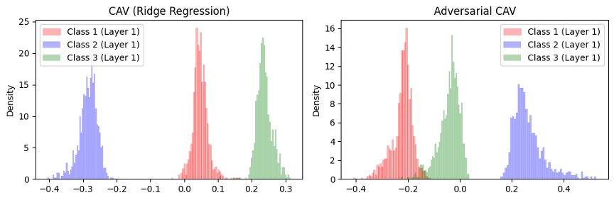
In the left panel (Ridge-Regression CAV),  aligns with the average direction from non-concept to concept, so the red, blue and green score-distributions are roughly evenly spaced around –0.3, 0 and +0.3, respectively, with similar variances.

In the right panel (Adversarial CAV),  is trained to distinguish clean vs. FGSM-perturbed concept examples. This “vulnerability” direction does not coincide with the original non-concept axis, causing:

• Concept collapse: Green class scores concentrate near zero.
• Inverted ordering: Blue class now peaks farthest right, even though it was a non-concept class.
• Unequal variances: Red class tightens up while blue widens, reflecting which class features overlap most with the adversarial direction.

Insight for natural disaster management: In wildfire monitoring, including daytime vs nighttime scenes as non-concept images can skew CAV toward illumination differences rather than smoke textures. In flood mapping, mixing riverine vs urban controls may hide true flood signatures. Carefully selecting or adversarially probing non-concept samples uncovers these biases.

Conclusion

By adapting CAVs to remote-sensing of wildfires and floods, we bridge human concepts (smoke, water) with deep model representations. Through both ridge and adversarial CAVs, combined with probabilistic analysis, practitioners gain fine-grained control over interpretability, enabling robust monitoring pipelines for natural disasters.

References

1. Been Kim et al. "Interpretability Beyond Feature Attribution: Quantitative Testing with Concept Activation Vectors (TCAV)". Proceedings of the 35th International Conference on Machine Learning (ICML). PMLR 80:2668-2677. 2018.
2. Frederik Pahde et al. "Navigating Neural Space: Revisiting Concept Activation Vectors to Overcome Directional Divergence". The Thirteenth International Conference on Learning Representations (ICLR). 2025.
3. Schnoor et al. “Concept Activation Vectors from a Statistical Learning Perspective”. Poster presentation at the 7th Joint Statistical Meeting of the Deutsche Arbeitsgemeinschaft Statistik (DAGStat 2025). 2025
4. Seddik et al. “Random Matrix Theory Proves that Deep Learning Representations of GAN-data Behave as Gaussian Mixtures”. Proceedings of the 37th International Conference on Machine Learning (ICML). PMLR 119:8573-8582. 2020.